Wishart distribution
| Parameters |  deg. of freedom (real) deg. of freedom (real) scale matrix ( pos. def) scale matrix ( pos. def) |
|---|---|
| Support |   positive definite matrices positive definite matrices |
 |
|
| Mean |  |
| Mode |  |
| Variance | 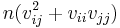 |
| CF |  |
In statistics, the Wishart distribution is a generalization to multiple dimensions of the chi-squared distribution, or, in the case of non-integer degrees of freedom, of the gamma distribution. It is named in honor of John Wishart, who first formulated the distribution in 1928.[1]
It is any of a family of probability distributions defined over symmetric, nonnegative-definite matrix-valued random variables (“random matrices”). These distributions are of great importance in the estimation of covariance matrices in multivariate statistics. In Bayesian inference, the Wishart distribution is of particular importance, as it is the conjugate prior of the inverse of the covariance matrix (the precision matrix) of a multivariate normal distribution.
Contents |
Definition
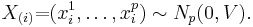
Suppose X is an n × p matrix, each row of which is independently drawn from a p-variate normal distribution with zero mean:
Then the Wishart distribution is the probability distribution of the p×p random matrix

known as the scatter matrix. One indicates that S has that probability distribution by writing
The positive integer n is the number of degrees of freedom. Sometimes this is written W(V, p, n). For n ≥ p the matrix S is invertible with probability 1 if V is invertible.
If p = 1 and V = 1 then this distribution is a chi-squared distribution with n degrees of freedom.
Occurrence
The Wishart distribution arises as the distribution of the sample covariance matrix for a sample from a multivariate normal distribution. It occurs frequently in likelihood-ratio tests in multivariate statistical analysis. It also arises in the spectral theory of random matrices and in multidimensional Bayesian analysis.
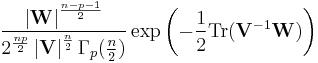
Probability density function
The Wishart distribution can be characterized by its probability density function, as follows.
Let W be a p × p symmetric matrix of random variables that is positive definite. Let V be a (fixed) positive definite matrix of size p × p.
Then, if n ≥ p, W has a Wishart distribution with n degrees of freedom if it has a probability density function given by
![p({\mathbf W}|{\mathbf V},n)=
\frac{
\left|{\mathbf W}\right|^{(n-p-1)/2}
\exp\left[ -\frac{1}{2} {\rm trace}({\mathbf V}^{-1}{\mathbf W})\right]
}{
2^{np/2}\left|{\mathbf V}\right|^{n/2}\Gamma_p(n/2)
}](/2012-wikipedia_en_all_nopic_01_2012/I/e31b47ac69538bb14b9be6494183e39f.png)
where Γp(·) is the multivariate gamma function defined as
![\Gamma_p(n/2)=
\pi^{p(p-1)/4}\Pi_{j=1}^p
\Gamma\left[ n/2%2B(1-j)/2\right].](/2012-wikipedia_en_all_nopic_01_2012/I/1e55030eac1604fa27c81800947dd8ed.png)
In fact the above definition can be extended to any real n > p − 1. If n ≤ p − 2, then the Wishart no longer has a density—instead it represents a singular distribution. [2]
Characteristic function
The characteristic function of the Wishart distribution is
In other words,
![\Theta \mapsto \operatorname{E}\left\{\mathrm{exp}\left[i\cdot\mathrm{trace}({\mathbf W}{\mathbf\Theta})\right]\right\}
=
\left|{\mathbf I} - 2i{\mathbf\Theta}{\mathbf V}\right|^{-n/2}](/2012-wikipedia_en_all_nopic_01_2012/I/1fe24d4c8174ca0b6192bbf21da30cfd.png)
where  denotes expectation. (Here
  and
and  are matrices the same size as
  ( is the identity matrix); and
  is the square root of −1).
Theorem
If  has a Wishart distribution with m degrees of freedom and variance matrix
  —write
  —and
—and  is a q × p matrix of rank q, then
Corollary 1
If  is a nonzero
  constant vector, then
  .
.
In this case,  is the chi-squared distribution and
  (note that
  is a constant; it is positive because is positive definite).
Corollary 2
Consider the case where 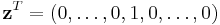 (that is, the jth element is one and all others zero). Then corollary 1 above shows that
gives the marginal distribution of each of the elements on the matrix's diagonal.
Noted statistician George Seber points out that the Wishart distribution is not called the “multivariate chi-squared distribution” because the marginal distribution of the off-diagonal elements is not chi-squared. Seber prefers to reserve the term multivariate for the case when all univariate marginals belong to the same family.
Estimator of the multivariate normal distribution
The Wishart distribution is the sampling distribution of the maximum-likelihood estimator (MLE) of the covariance matrix of a multivariate normal distribution with zero means. The derivation of the MLE involves the spectral theorem.
Bartlett decomposition
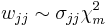
The Bartlett decomposition of a matrix W from a p-variate Wishart distribution with scale matrix V and n degrees of freedom is the factorization:
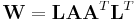
where L is the Cholesky decomposition of V, and:
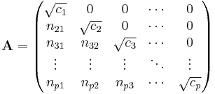
where  and
and  independently. This provides a useful method for obtaining random samples from a Wishart distribution.[3]
The possible range of the shape parameter
It can be shown [4] that the Wishart distribution can be defined if and only if the shape parameter n belongs to the set

This set is named after Gindikin, who introduced it[5] in the seventies in the context of gamma distributions on homogeneous cones. However, for the new parameters in the discrete spectrum of the Gindikin ensemble, namely,
the corresponding Wishart distribution has no Lebesgue density.
Relationships to other distributions
- The Wishart distribution is related to the Inverse-Wishart distribution, denoted by
 , as follows: If
  and if we do the change of variables
  , then
  . This relationship may be derived by noting that the absolute value of the Jacobian determinant of this change of variables is
  , see for example equation (15.15) in.[6]
 - The Wishart distribution is a conjugate prior for the precision parameter of the multivariate normal distribution, when the mean parameter is known.[7]
See also
References
- ^ Wishart, J. (1928). "The generalised product moment distribution in samples from a normal multivariate population". Biometrika 20A (1-2): 32–52. doi:10.1093/biomet/20A.1-2.32. JFM 54.0565.02.
- ^ “On singular Wishart and singular multivariate beta distributions” by Harald Uhling, The Annals of Statistics, 1994, 395-405 projecteuclid
- ^ Smith, W. B.; Hocking, R. R. (1972). "Algorithm AS 53: Wishart Variate Generator". Journal of the Royal Statistical Society. Series C (Applied Statistics) 21 (3): 341–345. JSTOR 2346290.
- ^ Peddada and Richards, Shyamal Das; Richards, Donald St. P. (1991). "Proof of a Conjecture of M. L. Eaton on the Characteristic Function of the Wishart Distribution,". Annals of Probability 19 (2): 868–874. doi:10.1214/aop/1176990455.
- ^ Gindikin, S.G. (1975). "Invariant generalized functions in homogeneous domains,". Funct. Anal. Appl., 9 (1): 50–52. doi:10.1007/BF01078179.
- ^ Paul S. Dwyer, “SOME APPLICATIONS OF MATRIX DERIVATIVES IN MULTIVARIATE ANALYSIS”, JASA 1967; 62:607-625, available JSTOR, or here.
- ^ C.M. Bishop, Pattern Recognition and Machine Learning, Springer 2006.